The objective of this case study is to determine the torsional stress function \( \Psi \) present in a bar of unit square cross-section that is fully constrained at one end and subjected to a small twisting moment at the other end. The twisting moment is applied about an axis perpendicular to the square section. The bar is subject to no other external forces. The stress function is determined at discrete points using the finite difference method.
A comparison is made with the results from a finite element calculation (presented by J.N. Reddy) for the same problem. A color plot of the results for one quadrant of the square section is displayed in Figure 1 to the right. The Fortran source code that is used for the analysis is also available.
It can be shown that the stress function satisfies the 2-d Poisson's equation over the square domain \( \Omega \) $$ \begin{equation} \nabla^2 \Psi = -2 \space\space \text {in} \space\space \Omega \label{eq:eq1} \end{equation} $$ and that the stress function vanishes on the boundary \( \Gamma \). $$ \begin{equation} \Psi = 0 \space\space \text {on} \space\space \Gamma. \label{eq:eq2} \end{equation} $$
Noting that \( \Psi \) is symmetric about the x- and y-axes, it is necessary only to consider a single quadrant of the square cross-section. In this case, the (+x,+y) quadrant is modeled (see Figure 2). The symmetry anout the x- and y-axes allows the following boundary conditions to be prescribed for the single quadrant. $$ \begin{equation} \begin{aligned} \frac{\partial \Psi}{\partial x} = 0 \space\space \text {on} \space\space x \text{=0}\\ \\ \frac{\partial \Psi}{\partial y} = 0 \space\space \text {on} \space\space y \text{=0} \end{aligned} \label{eq:eq3} \end{equation} $$ The boundary condition on the remainder of the boundary states that \(\Psi\) vanishes there. $$ \begin{equation} \Psi = 0 \space\space \text {on} \space\space x \text{=1 and} \space y \text{=1} \label{eq:eq4} \end{equation} $$ The finite difference grid used for this example is a simple 8x8 lattice of points equally spaced by a distance \( h \) = 0.125. The grid points are indexed with increasing \(i\) in the \(x\)-direction and increasing \(j\) in the \(y\)-direction with (\(i\),\(j\)) = (0,0) located in the bottom left hand corner. A finite difference approximation for equation \eqref{eq:eq1} employs the 2nd order central difference formula for \(\nabla^2 \Psi\) and is expressed as follows: $$ \begin{equation} \Psi_{i+1,j} + \Psi_{i-1,j} + \Psi_{i,j+1} - 4\Psi_{i,j} + \Psi_{i,j-1} = -2 \space h^2 = - \tfrac{1}{128}. \label{eq:eq0} \end{equation} $$ The finite difference approximation in equation \eqref{eq:eq0} suggests the following five-point stencil. $$ \begin{equation} \begin{bmatrix} &\space1& \\ 1&-4&\space1 \\ &\space1& \end{bmatrix} \boldsymbol{\Psi} = - \tfrac{1}{128}. \label{eq:eq5} \end{equation} $$ The Neumann boundary conditions imposed on the x- and y- axes can be implemented with the use of ghost points. $$ \begin{equation} \begin{aligned} \frac{\partial \Psi}{\partial x} = 0 \space\space\implies\space\space \Psi_{-1,j} = \Psi_{1,j} \space\space\space\space j = 0, .. ,7\\ \\ \frac{\partial \Psi}{\partial y} = 0 \space\space\implies\space\space \Psi_{i,-1} = \Psi_{i,1} \space\space\space\space i = 0, .. ,7 \end{aligned} \label{eq:eq6} \end{equation} $$ When fully assembled, the following matrix equation represents the finite difference approximation for the entire system. $$ \begin{equation} \begin{bmatrix} B&2I&&&&& \\ I&B&I&&&& \\ &&&\ddots&&& \\ &&&&\ddots&& \\ &&&&I&B&I \\ &&&&&I&B \end{bmatrix} \begin{bmatrix} \boldsymbol{\Psi_{0,0:7}} \\ \boldsymbol{\Psi_{1,0:7}} \\..\\..\\ \boldsymbol{\Psi_{6,0:7}} \\ \boldsymbol{\Psi_{7,0:7}} \end{bmatrix} = - \tfrac{1}{128} \begin{bmatrix} \mathbf{1}\\\mathbf{1}\\..\\..\\\mathbf{1}\\\mathbf{1} \end{bmatrix} \label{eq:eq7} \end{equation} $$ in which \(\mathbf{1}\) is an 8x1 column vector with entries equal to 1.0, \(I\) is the 8x8 identity matrix and $$ \begin{equation} B = \begin{bmatrix} -4&\space2&&&&& \\ \space1&-4&\space1&&&& \\ &\space1&-4&1&&& \\ &&&\ddots&&& \\ &&&\space1&-4&\space1& \\ &&&&\space1&-4&\space1 \\ &&&&&\space1&-4 \end{bmatrix} \label{eq:eq8} \end{equation} $$
The C++ source code that accompanies this case study solves for \(\Psi_{i,j}\) by calling the LAPACK function DGBSV to perform a solution of \eqref{eq:eq7}, wherein the bandedness of the matrix on the LHS is expressed in a specific format given in the LAPACK documentation: LAPACK banded matrix format
The Fortran source code that accompanies this case study solves for \(\Psi_{i,j}\) by calling the Intel(R) Math Kernel Library version of Pardiso to perform an LU-factorization of the sparse, real and non-symmetric matrix written on the left hand side of equation \eqref{eq:eq7}. The source code uses 3-array CSR format to specify the values and topology for this matrix.
It should be noted that an iterative approach such as the Jacobi Method could just as easily be used. At iterative approach might prove particularly useful for larger systems wherein parallel programming constructs could be desirable.
A comparison is now made against the results provided for the same problem by J.N. Reddy1 (see Example 8.8). The results presented for the 4x4 mesh of quadratic elements are particularly useful as they provide predictions for \(\Psi\) that coincide with the analytical solution to equation \eqref{eq:eq1} to within 5 significant d.p. The comparison is made between the \(\Psi\) result from Reddy and the finite difference method presented here for selected locations in the (+x,+y) quadrant. The prediction for \(\Psi\) at (0,0) is accurate to 2 significant d.p.
| \(\Psi_{i,j}\) | \(x\) | \(y\) | \(\Psi_{Reddy}\) | \(\Psi_{FDM}\) |
| \(\Psi_{0,0}\) | 0.0 | 0.0 | 0.14734 | 0.14689 |
| \(\Psi_{2,4}\) | 0.125 | 0.25 | 0.1089 | 0.1086 |
| \(\Psi_{4,4}\) | 0.25 | 0.25 | 0.09057 | 0.09025 |
| \(\Psi_{6,4}\) | 0.375 | 0.25 | 0.05636 | 0.05614 |
Reference: 1. Reddy, J. N.: An Introduction to the Finite Element Method, 2nd ed., McGraw-Hill
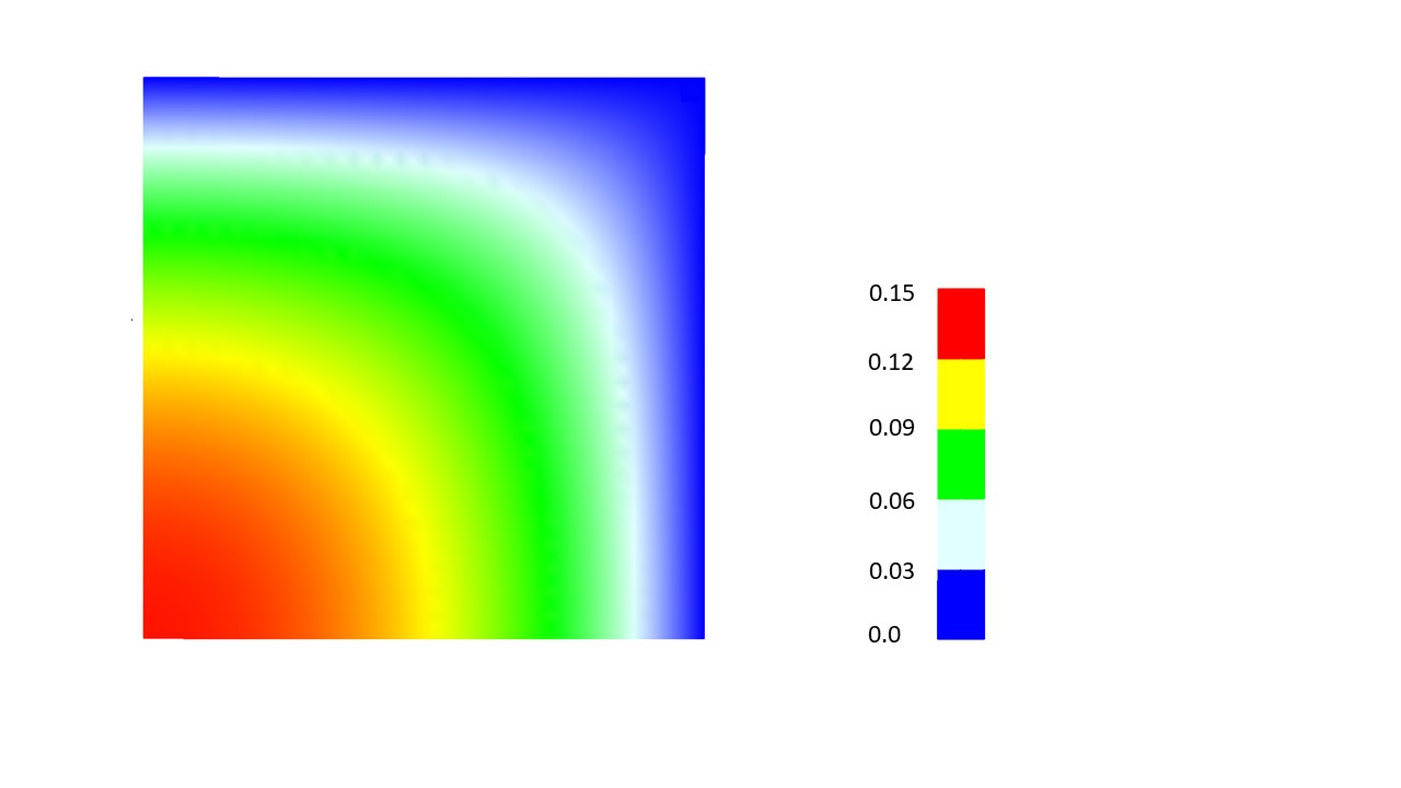
Figure 1 - Stress Function \( \Psi \) over (+x,+y) quadrant
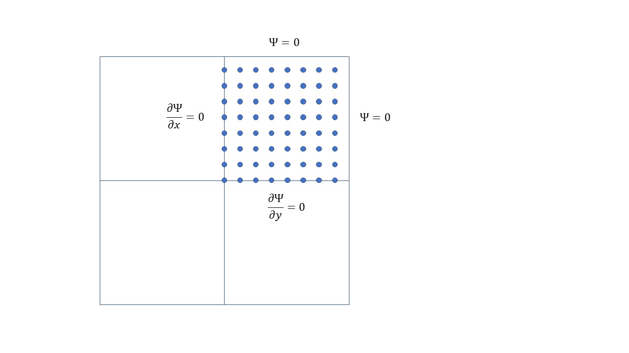
Figure 2 - Finite difference grid with boundary conditions
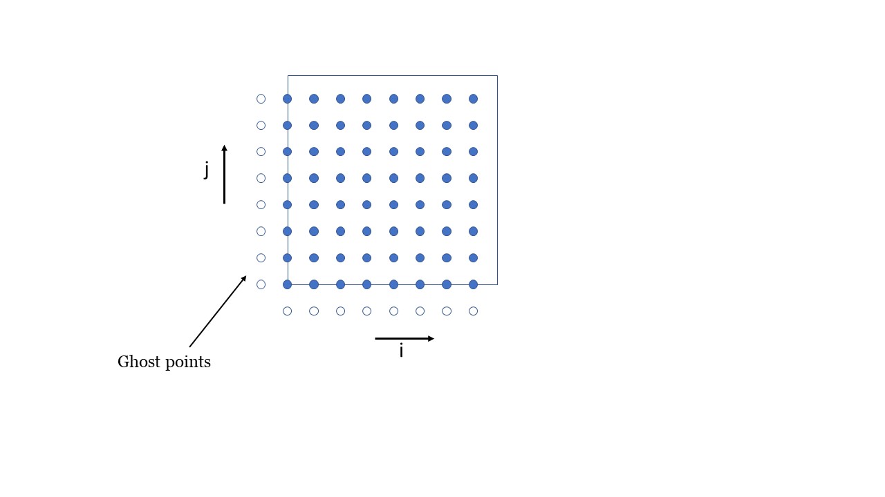
Figure 3 - Finite difference grid with ghost points